
Simulation is a very potent tool that is often lacking in many data scientists’ toolkits. In this article, I will teach you how to use simulation in combination with other analytical tools.
I will be sharing some educational and professional examples of simulation with Python code. If you are a data scientist (or on the road to becoming one), you’ll love the possibilities that simulation opens for you.
What is simulation?
Simulating is digitally running a series of events and recording their outcomes. Simulations help us when we have a good understanding of how individual events work, but not of how the aggregate works.
In physics, simulations are often used when we have a hard-to-solve differential equation. We know the starting state, and we know the rules for infinitesimal (very small) changes, but we don’t have a closed formula for longer timespans. Simulation allows us to project that initial state into the future, step by step.
In data science, we usually work with probabilistic events. Sometimes we can easily aggregate them analytically. Other times there is no analytical solution, or it’s very hard to reach it. We can estimate the probabilities and expected results of complex chains of events, by running multiple simulations and aggregating the results. This can be very useful to understand the risks we are exposed to.
Simulation is also used in hard artificial intelligence. When interacting with others, simulation can allow us to anticipate their behavior and plan accordingly. For example, Deep Mind’s Alpha Go uses simulations to calculate some moves into the future and make a better assessment of the best moves in its current position.
To run a simulation we will need a model of the underlying events. This model will tell us what can happen at any given point, the probabilities of each outcome and how we should evaluate the results.
The better our model, the better the accuracy of the simulation. However, simulations with imperfect models can still be helpful and give us a ballpark estimate.
Simulation is a subject where examples work better than theory, so let’s jump into some use cases.
Example 1. Estimate the value of pi by using simulation
This task can be done in many ways. One of the easiest is as follows:
- Draw a square of side 2 and with its center at the origin of coordinates of a 2d plane
- Draw the inscribed center of that square (radius 1 and its center at the origin of coordinates)
- Sample random points from the square (two uniform distributions from -1 to 1)
- Whenever you draw a point, check whether it is inside the circle or not
- The proportion of points inside the circle will be proportional to the area of the circle so:
![\[{Num\_points\_inside\_circle \over Num\_total\_points} \approx {Area\_of\_circle \over Area\_of\_square} = {\pi \cdot 1^2 \over 2 \cdot 2} = {\pi \over 4}\]](https://oriolcosp.com/wp-content/ql-cache/quicklatex.com-235261e0b5e92ba191988d05f6ebbf80_l3.png "Rendered by QuickLaTeX.com")
And finally:
![\[\pi \approx 4 \cdot {Area\_of\_circle \over Area\_of\_square}\]](https://oriolcosp.com/wp-content/ql-cache/quicklatex.com-0f31b971f9f5e88c801186ee7416f2e1_l3.png "Rendered by QuickLaTeX.com")
Here is Python code to simulate the value of pi:
import numpy as np
import matplotlib.pyplot as plt

np.random.seed(1234)

num_sims = 5000
x_random = np.random.rand(num_sims)
y_random = np.random.rand(num_sims)

inside_circle = ((x_random ** 2 + y_random**2) < 1)

print(4*inside_circle.mean())
plt.figure(figsize=[8,5])
n_to_one = np.arange(1, num_sims+1)
plt.plot(n_to_one , 4*inside_circle.cumsum() / n_to_one)
plt.show()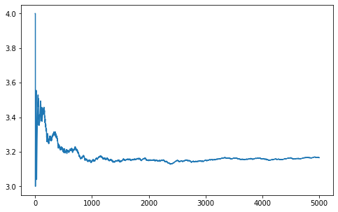
Similar methods can be used to estimate the value of integrals via simulation.
Example 2. Solve a difficult probability problem
Solve this problem by P. Winkler:
One hundred people line up to board an airplane. Each has a boarding pass with an assigned seat. However, the first person to board has lost his boarding pass and takes a random seat. After that, each person takes the assigned seat if it is unoccupied, and one of the unoccupied seats at random otherwise. What is the probability that the last person to board gets to sit in his assigned seat?
The problem can be solved using logic and probabilities, but it can also be solved by simply programming the described behavior and running some simulations:
import numpy as np
import matplotlib.pyplot as plt

np.random.seed(1234)

def simulate_boarding(num_passengers):
    passenger_seats = set(range(num_passengers))
    for i in range(num_passengers):
        if i == num_passengers - 1:
            if list(passenger_seats)[0] == i:
                return 1
            else:
                return 0
        if (i == 0) or (not i in passenger_seats):
            i = list(passenger_seats)[np.random.randint(0, num_passengers - i)]
            passenger_seats.remove(i)
        else:
            passenger_seats.remove(i)

num_sims = 10000
num_passengers = 100
positives = 0

is_same_seat = [simulate_boarding(num_passengers) for i in range(num_sims)]
is_same_seat = np.array(is_same_seat)


print(is_same_seat.mean())
plt.figure(figsize=[8,5])
one_to_n = np.arange(1, num_sims+1)
plt.plot(one_to_n, is_same_seat.cumsum() / one_to_n)
plt.show()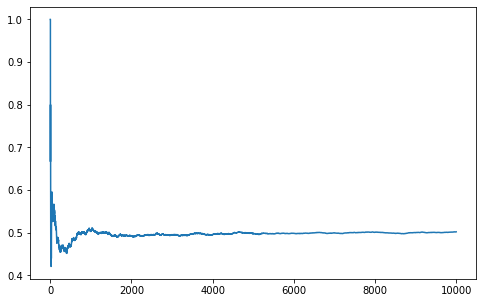
You can find more probability problems to practice here.
Example 3. Simulating game outcomes
How many games would it take Magnus Carlsen (Elo of 2847 as of 18-07-2021) to get back to his current rating if he was dropped at 1000?
To solve this problem we need to understand how the Elo system works.
First, given two player’s Elo ratings, the probability of player1 beating player2 is:
![\[P(\textrm{player1 beats player2}) = {1 \over 1 + K \cdot 10 ^{(Elo_2 - Elo_1)/400}}\]](https://oriolcosp.com/wp-content/ql-cache/quicklatex.com-33d9fbc23e66c26c6357263352a56c99_l3.png "Rendered by QuickLaTeX.com")
Second, after the game, player1’s Elo rating is updated as follows:
![\[Elo_1= Elo_1+K \cdot (\textrm{result} - P(\textrm{player1 beats player2}))\]](https://oriolcosp.com/wp-content/ql-cache/quicklatex.com-edfd9b04dfd4f3c46c65487ef638072b_l3.png "Rendered by QuickLaTeX.com")
Where:
- result is 1 for a win, 0.5 for a tie and 0 for a loss
- K (also known as K-factor) is the maximum possible adjustment per game and varies depending on the player’s age, games played and ELO
Now that we have a model, we just have to initialize Magnus current Elo to 1000 and code a while loop that:
- Has Magnus play a game against a player of his current Elo
- Calculates the probability of winning using the real Elo and simulates the outcome of the game
- Updates Magnus’s current Elo according to the result
- Stops the loop if Magnus has reached his real Elo
import numpy as np
import matplotlib.pyplot as plt
np.random.seed(1234)
def get_prob(elo1, elo2):
return 1/(1+10**((elo2 - elo1)/400))
def update_elo(elo, prob, result, k):
return elo + k * (result - prob)
def play_until_top(real_elo, initial_elo):
current_elo = initial_elo
num_games = 0
k = 40
elo_list = [initial_elo]
while current_elo < real_elo:
if num_games > 30:
k = 20
if current_elo > 2400:
k = 10
prob_win = get_prob(real_elo, current_elo)
result = 1 if np.random.rand(1)[0] < prob_win else 0
current_elo = update_elo(current_elo, 0.5, result, k)
elo_list.append(current_elo)
num_games += 1
return elo_list
num_sims = 1000
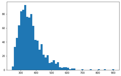
num_games = [len(play_until_top(2847, 1000)) for i in range(num_sims)]
num_games = np.array(num_games)
print(num_games.mean())
plt.figure(figsize=[8,5])
plt.hist(num_games,bins=50)[2]
elo_history = np.array(play_until_top(2847, 1000))
plt.figure(figsize=[8,5])
plt.plot(np.arange(0, len(elo_history)), elo_history)
plt.show()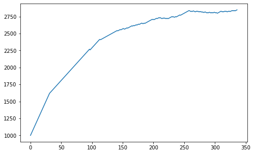
Another cool example would be to simulate the NBA playoffs. For a first approach, you can assume that each team has a probability of winning proportional to the games they won during the regular season (GW) so that in any game the probability of team 1 winning is GW1 / (GW1 + GW2). You can also analyze how probabilities change if you change the series from Best of 7 to Best of 5 or Best of 9.
Example 4. Business application, estimating value at risk
Collectors LTD is a debt collection company focused on enterprise debt. It buys portfolios of business loans that have defaulted at some point and tries to collect the payments for those loans. Some of the companies will be bankrupt and won’t be able to pay, and others are likely to go bankrupt in the future. The key to Collectors LTD’s business is in estimating the value it can get back from a portfolio. For this reason, Collectors LTD has developed a model that predicts the probability of a company repaying part of that debt. Among those companies that repay some of the debt, the amount paid is distributed uniformly from 0% to 100%. Collectors LTD can use its model in combination with simulation to evaluate the expected return of the portfolio, and how volatile that return is.
Since I can’t share the real data with you, I’ve created a synthetic dataset that mimics the relevant properties:
import numpy as np
import matplotlib.pyplot as plt

np.random.seed(1234)

def generate_synthetic_portfolio(num_companies):
    debt = 100000 * np.random.weibull(0.75, num_companies)

    prob_repayment = np.random.normal(0.2, 0.1, num_companies)
    prob_repayment = np.clip(prob_repayment, a_min=0, a_max=1)

    return debt, prob_repayment

num_companies = 1000
debt, prob_repayment = generate_synthetic_portfolio(num_companies)
Given the following synthetically generated portfolio, estimate the expected amount to be collected and the 95% percentile.
def simulate_collection(debt, prob_repay):
    num_companies = len(debt)
    did_repay = (np.random.rand(num_companies) < prob_repay)
    pct_paid = np.random.rand(num_companies)
    amount_collected = debt * did_repay * pct_paid
    return amount_collected.sum()

num_sims = 1000
amount_collected =
    np.array([simulate_collection(debt, prob_repay) for i in range(num_sims)])

print(f"Total debt: {np.round(amount_collected.mean())} usd")
print(f"Average amount collected: {np.round(amount_collected.mean())} usd")
percentile_95 = np.round(np.sort(amount_collected)[int(0.05*num_sims)])
print(f"95% percentile collection: {percentile_95} usd")

plt.figure(figsize=[8,5])
plt.hist(amount_collected,bins=50)[2]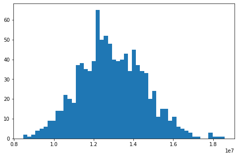
Keep in mind that this solution assumes the probabilities of collection are independent of one another. This isn’t true for systemic risks such as a global economic downturn.
Conclusion
I hope you’ve liked these examples and that you can find applications of simulation in your day-to-day data science job. If you’ve enjoyed the article, please subscribe and share it with your friends.